This is a companion report to the GIS For Conservation eMedia project, published with Unitec ePress. Unitec ePress periodically publishes Research Reports supporting eMedia publications providing evidence and contextual analysis, authored by members of staff and their research associates. All reports and eMedia are blind reviewed. Click here to read the pdf, or read the html version below.
GIS For Conservation
Using Predicted Locations and an Ensemble Approach to Address Sparse Data Sets for Species Distribution Modelling: Long-horned Beetles (Cerambycidae) of the Fiji Islands
Authors
Glenn D. Aguilar, Environmental and Animal Sciences, Unitec Institute of Technology
Hilda Waqa-Sakiti, South Pacific Herbarium, University of the South Pacific
Linton Winder, Forestry and Resource Management, Toi-Ohomai Institute of Technology
Abstract
Several modelling tools were utilised to develop maps predicting the suitability of the Fiji Islands for long-horned beetles (Cerambycidae) that include endemic and endangered species such as the Giant Fijian Beetle Xixuthrus heros. This was part of an effort to derive spatially relevant knowledge for characterising an important taxonomic group in an area with relatively few biodiversity studies. Occurrence data from the Global Biodiversity Information Facility (GBIF) and bioclimatic variables from the WorldClim database were used as input for species distribution modelling (SDM). Due to the low number of available occurrence data resulting in inconsistent performance of different tools, several algorithms implemented in the DISMO package in R (Bioclim, Domain, GLM, Mahalanobis, SVM, RF and MaxEnt) were tested to determine which provide the best performance. Occurrence sets at several distribution densities were tested to determine which algorithm and sample size combination provided the best model results. The machine learning algorithms RF, SVM and MaxEnt consistently provided the best performance as evaluated by the True Skill Statistic (TSS), Kappa and Area Under Curve (AUC) metrics. The occurrence set with a density distribution of one sampling point per 10km2 provided the best performance and was used for the final prediction model. An ensemble of the best-performing algorithms generated the final suitability predictive map. The results can serve as a basis for additional studies and provide initial information that will eventually support decision-making processes supporting conservation in the archipelago.
Introduction
In many high-biodiversity areas of the world, species occurrence data often arises from numerous surveys spanning decades, with limited or inaccurate location information (particularly from surveys gathered before the availability of global positioning systems). Such data is challenging when attempts are made to characterise the spatial distribution of species (Hernandez et al., 2006). Modelling provides a useful approach to overcome these problems and can be utilised to provide information for conservation planning and management purposes (Rodriguez et al., 2007; Guisan et al., 2013). This is particularly important for island countries such as Fiji where land-use conflicts, population pressure, management considerations, and the effects of climate change amplify existing and continuing threats to existing biodiversity (Warner, 2000; Lambin & Meyfroidt, 2011; Higgins, 2007; Cayuela, 2004; Faleiro et al., 2013).
To contribute to the information needs of conservation management, Species Distribution Modelling (SDM) has become a well-established approach in predicting the suitability of defined areas for selected species. Also known as Ecological Niche Models, Habitat Suitability Models or Climate Envelope Models, SDM uses environmental data at species occurrence sites to predict or produce values that represent the suitability of the area for the species or group of species. SDM has become a mainstream method used for biodiversity conservation and planning purposes (Guillera-Arroita et al., 2015; Duan et al., 2014). It may be used to identify areas that should be prioritised when resources or expertise for field studies are limited, with the map outputs providing initial guidance on the potential distribution of target taxa (Raxworthy et al., 2003). SDM has also been used to predict alien species invasion and proliferation (Roura-Pascual et al., 2008; Poulos et al., 2012; Thuiller & Richardson, 2005); identify areas for the conservation of threatened and/or endangered species (Bombi et al., 2009; Puschendorf et al., 2009; Wilson et al., 2007; Nabout et al., 2010); and map areas for biofuel production (Evans et al., 2010). SDM was also used to investigate poorly sampled but species-rich localities (Fitzpatrick et al., 2011), in order to determine areas for follow-up surveys to try to find new populations (Oleas et al., 2014). Another increasing use of SDM is the projection of species spatial distribution into different geographic locations and into future and past climate conditions using relevant environmental data such as global circulation, land cover and climate scenarios (Feeley et al., 2013; Yates et al., 2009).
At its early adoption and development stages, SDM mainly relied on the application of one technique or algorithm. The choice of modelling tool depended on the author’s involvement in its development, the availability of environmental and species occurrence data, tool performance, computing processing costs and training of users (Stohlgren et al., 2010). Comparative efforts have demonstrated performance differences between algorithms, leading to the recommendation that an ensemble (or consensus) approach based on the evaluation of results from a set of different algorithms or models be used (Araujo & New, 2007; Marmion et al., 2009). An ensemble addresses the weakness of each individual algorithm and, using performance as a weighting value, allows the determination of a model’s contribution to the final predictive map. Ensemble modelling has been used for single- and multi-species distribution analyses (Fitzpatrick et al., 2011), invasive species (Stohlgren et al., 2010; Poulos et al., 2012; Roura-Pascual et al., 2008), rare and endangered species prediction (Evangelista et al., 2008; Bombi et al., 2009), and forecasting distributions with climate change scenarios (Jarnevich & Stohlgren, 2009). Several software tools such as ModEco (Guo & Liu, 2010), openModeller (Souza, Munoz et al., 2009) as well as the R packages of BIOMOD (Thuiller et al., 2009), DISMO (Hijmans et al., 2013) and SDM (Naimi & Araujo, 2016) allow the production of ensembles from different algorithms.
Inherent in data not systematically sampled is the problem of spatial autocorrelation where clusters of occurrences result in degradation of the model’s ability to predict because of environmental biases (Veloz, 2009). By increasing the sample size and explicit spatial filtering of presence data, omission and commission errors in some modelling tools are proven to be minimised and result in improved model performance (McPherson et al., 2004; Kramer-Schadt et al., 2013) as measured by commonly-used indicators including the AUC, Kappa and TSS (Duan et al., 2014; Allouche et al., 2006). These provide measures of performance for each model, enabling a comparison of the different algorithms. Together with the measurement of consistency, the evaluation of performance determined which model or group of models to use for all stages of the modelling process (Wisz et al., 2008).
Whilst insects dominate the biodiversity of the animal kingdom, the majority of modelling work has focused on vertebrates and plants (Tognelli et al., 2009). Studies on insects include those that focus on human disease vectors (Peterson et al., 2005), introduced and invasive species (Roura-Pascual, 2008) and the biodiversity conservation of species vulnerable to climate change (Meggs et al., 2004; Sauer et al., 2011; Jarnevich & Stohlgren, 2009). The lack of reliable taxonomic and biogeographic information regarding insects is the main factor preventing the development of SDMs for conservation purposes (Tognelli et al., 2009; Chefaoui et al., 2005). In the Fiji Islands, where conservation planning to protect a host of endemic and endangered species – including rare insect species – is gaining ground, a series of workshops aimed at developing the modelling and GIS capabilities for researchers at the South Pacific Herbarium provided the opportunity to develop models for different indicator species of importance to the area.
For this study, we used data from the Fiji Islands available on Cerambycidae to:
(i) tackle the problem of sparse occurrence data whilst utilising information that was available;
(ii) use an ensemble approach to provide guidance on the performance of a range of modelling tools;
(iii) produce a suitability map for Cerambycidae throughout the archipelago in order to support the establishment of conservation priorities in a country where relatively few insect biodiversity studies have been completed.
Methods
SDM tools require two types of data: species occurrence with location consisting of longitude and latitude, and environmental or bioclimatic characteristics at each of the location points. The SDM algorithm then generates a model that is used to develop a predictive map of suitability for the entire study area. Some algorithms require absence data while others will work with presence-only data (which may require the generation of ‘pseudo-absences’ for evaluation of model performance). For this study, two stages of modelling were undertaken. Firstly, the inherent scarcity and spatial autocorrelation of survey-generated data was addressed. Original occurrence points based on Cerambycidae data were sourced from the Global Biodiversity Information Facility (GBIF, 2015), and processed using an ensemble-based approach to generate sets of predicted occurrences. Secondly, the resulting predicted presence sites at different distribution densities were used to generate a suitability map for Cerambycidae for the Fiji Islands (Figure 1.) (http://www.gbif.org/ accessed in October 2015) and processed using an ensemble-based approach to generate sets of predicted occurrences.
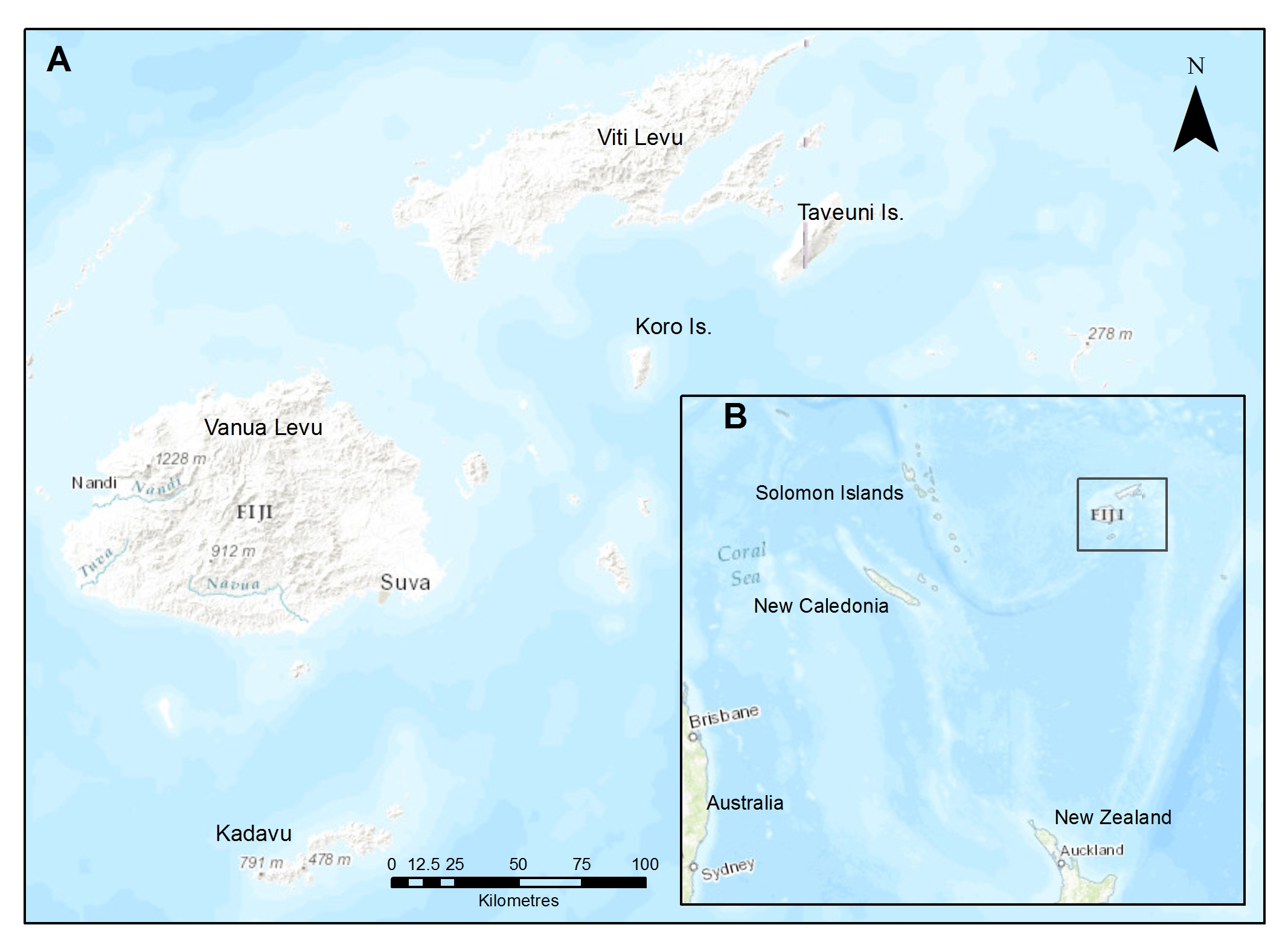
Figure 1. Study location is in Fiji, (A) consisting of the largest islands Vanua Levu and Viti Levu, located in the Southwest Pacific (B).
The original 24 data points were processed using ArcMap v10.2 to check for duplication and spatial autocorrelation, using the spatially rarefied tool of the SDMtoolbox (Brown, 2014). This step reduces the bias associated with the clustering of occurrence points and the tendency of models to exhibit spatial autocorrelation, reduces sampling bias, and improves and enhances model performance (Boria et al., 2014; Fourcade et al., 2014; Veloz, 2009; Hijmans et al., 2012). Recommendations on the minimum number of sampling locations necessary to produce consistent and reliable results range from five to 200, with higher values contributing to better performance (Hernandez et al., 2006; Stockwell & Peterson, 2002; Wisz et al., 2008;). However, Wisz et al. (2008) reported a lack of consistent performance among several algorithms when sample size is less than 30.
Data available from WorldClim (Hijmans et al., 2005) was used as environmental layers. The current WorldClim scenario dataset consists of 19 variables interpolated from the average of 50-year records collected from 1950 to 2000, and consists of 11 temperature- and eight precipitation-related variables. The resolution chosen was the highest available at 30 arc seconds (a resolution of approximately a kilometre per pixel). Processing the environmental layers involved the use of ArcMap and included transforming the projection from WGS84 into the Fiji Map Grid 86. This was required in order to display the Fiji Islands as one entity, because the presence of the International Dateline through the archipelago split the islands, and the GIS software placed them by default at opposite ends of the map. To check for cross-correlation and minimise multi-collinearity within the variable set, highly correlated variables were identified using the SDMtoolbox in ArcMap (Dormann et al., 2013; Brown, 2014), and variables with Pearson correlation coefficient values less than -0.7 or greater than 0.7 were omitted from the modelling.
The DISMO package in R (Hijmans et al., 2013; Hijmans & Elith, 2016) was utilised for species distribution modelling. Seven tools were used for modelling the distribution, one of which is a regression model (GLM), three are profile methods (Bioclim, Domain and Mahalanobis) and three are machine-learning methods (randomForest, MaxEnt, and SVM).
GLM (Generalised Linear Model) applies ordinary least squares regression in model fitting, using maximum likelihood that allows the magnitude of the variance of measurements to be functions of predicted values. GLM uses a logit link function to generate relationships between environmental variables and the probability of presence or absence of a species at a location (Guisan, Edwards & Hastie, 2002; Rushton et al., 2004). GLM is suited for ecological data that is not normally distributed (Guisan et al., 2002). GLMs generally outperform simpler methods, and are widely used in ecological studies (Ferrier & Watson, 1997; Brotons et al., 2004).
Bioclim is one of the first and one of the most widely-used algorithms for species distribution modelling. Described as a ‘climate-envelope-model’, Bioclim computes the suitability of a geographic location for a species by a comparison of the environmental variables at any locations to a percentile distribution of the variables at known occurrence sites (Booth et al., 2014). Bioclim was found to be outperformed by more recent algorithms, particularly in climate change modelling (Hijmans & Graham, 2006), but it is still used because it is easy to understand and therefore useful for instructional purposes, or for introducing species distribution modelling (Hijmans & Elith, 2016).
Domain (Carpenter et al., 1993) uses the Gower distance between environmental variables at any geographic location and the location of known occurrences. Domain assigns a classification value of habitat suitability to each location to determine the boundaries of the ecological niche of a species (Duan et al., 2014). Performance of Domain with small sample sizes was in the intermediate range when compared to other commonly-used algorithms (Elith et al., 2006).
The algorithm based on the Mahalanobis distance (Mahalanobis, 1936) is a traditionally-used approach for satellite imagery classification (Foody et al., 1992) but has also been applied in SDM (Hernandez et al., 2006). Mahalanobis distance does not depend on the scale of measurements, and ranks the potential sites through their Mahalanobis distance to a vector that relates to the mean values of all recorded environmental factors. A set distance threshold determines the ecological niche boundaries and an elliptical envelope is produced to describe the interaction between environmental variables (Cheaib et al., 2012).
RandomForest (RF) is both a regression and classification model (Breiman, 2001) and is the machine-learning version of Classification and Regression Trees (CART) (Breiman et al., 1984). RF grows an ensemble of decision trees using a random selection of subsets of occurrence data and environmental variables. The algorithm determines the final tree or classification, based on the average of all trees. Consistency and relatively superior performance is a reported characteristic of RF when used in SDM (Fukuda et al., 2013; Duan et al., 2014).
Based on the machine-learning algorithm called maximum entropy, MaxEnt models the distribution of a species over a defined area, based on the premise that its spread is as close as possible to a uniform distribution (Phillips et al., 2006). MaxEnt is widely used in SDM (Fourcade et al., 2014), generally has better performance compared to other models (Elith et al., 2006), and may be used in a wide variety of applications such as modelling stray cat distributions (Aguilar et al., 2015) and invasive species modelling (Liang et al., 2014).
SVM or the Support Vector Machine algorithm is a generalised linear classifier based on the Vapnik-Chervonenkis (VC) dimension and the structural risk minimisation theory (Burges, 1998). First used in SDM to describe sudden oak death in California (Guo et al., 2005), it has found widespread use due to its simplicity and performance (Drake et al., 2006; Duan et al., 2014).
While Bioclim and Domain can use presence-only data in modelling, the regression method GLM and machine-learning based methods (Philipps et al., 2006) use absence data (which can be substituted with background data in cases where absence data is not available). We used the DISMO random sampling function to generate a set of background points used in modelling and in the evaluation of model performance (Hijmans & Elith, 2016).
An initial run of all seven models was conducted using the original 24 presence points to derive a set of occurrence points based on different distribution densities. We used the AUC, Kappa and TSS criteria to select the best-performing models. The area under the ROC curve (AUC) is used extensively in species distribution modelling to evaluate model performance (Elith et al., 2006; Phillips et al., 2006). The ROC curve plots the rate of observed presences correctly predicted or True Positives Rate (TPR or sensitivity) and the proportion of observed absences incorrectly predicted or false positive or FPR (False Positive Rate which is 1 – specificity or True Negative Rate, TNR). The AUC determines the predictive performance of a model (Swets, 1988). Values of the AUC ranged from 0 to 1 where I indicates high performance, values of AUC less than 0.7 are considered to have lower performance and a value of 0.5 no better than random (Luoto et al., 2006; Roura-Pascual et al., 2009). A high AUC score showed that the model was able to distinguish, at a high level of accuracy, the locations where the species were present or absent. The AUC is also interpreted as the probability of a model distinguishing between a presence record and an absence record if each record is selected randomly from the set of presences and absences. (Fielding & Bell, 1997; Pearce & Ferrier, 2000). AUC is a test that ideally employs both presence and absence records, but methods have effectively used ‘pseudo-absence’ records instead of observed absences (Phillips et al., 2006). Since the available data is only presence data, we used a routine in R to produce pseudo absences, enabling the model evaluation routines of the algorithms to run (Hijmans & Elith, 2016).
Aside from AUC, the other measure commonly used to evaluate model performance and included in the packaged DISMO is Kappa (Cohen, 1960). Kappa measures the agreement between observed and predicted values, taking into account the correct predictions expected by chance. Kappa values range from -1 to +1 with values less than 0 indicating a performance that is not better than random. Values of Kappa nearing +1 indicate high performance and it is one of the most popular measures for presence-absence predictions (Pearson, Dawson & Liu, 2004; Segurado & Araujo, 2004).
Another commonly-used performance metric is the True Skill Statistic, TSS (Allouche et al., 2006). TSS is calculated using the TPR and TNR with values ranging from 0 to 1 with 0 no better than random and 1 indicating perfect model agreement (Domisch et al., 2013). TSS retains all the advantages of Kappa while addressing Kappa’s sensitivity to prevalence (Allouche et al., 2006). Showing the results of AUC, Kappa and TSS as performance measures all together provides greater confidence in model results and provides a better evaluation compared to reliance on a single statistic (Lobo et al., 2008; Jarnevich et al., 2015).
For the first run to generate the greater number of occurrence points, a value of 0.9 for AUC and TSS/Kappa of less than 0.4 was used as the cut-off for the model to be used. For the next stage with the new set of occurrence points, models with AUC values greater than 0.9 and TSS or Kappa greater than 0.4 were used for selecting the final ensemble (Zhang et al., 2015).
Predicted suitability maps of the best-performing models based on AUC, Kappa and TSS were ensembled to develop a final predicted suitability for Cerambycidae. This map of suitability was then thresholded using the average maximum TNR + TPR of the models to produce a simple presence and absence map (Liu, White & Newell, 2013). The presence raster of the resulting thresholded image was then converted into a point shapefile to represent and provide the longitude and latitude of the occurrence point of the species for the next stage in modelling. These points were rarefied using the rarefy tool of the SDMtoolbox in ArcMap (Brown, 2014) at distribution densities of one occurrence per 5, 10, 20 and 50 square kilometres with the resulting points used as input sets for the next stage of modelling. This process resulted in increased sample sizes that addressed concerns of sparse data sets as well as autocorrelation of clustered occurrence points (MacPherson et al., 2004; Hernandez et al., 2006). Model stability or consistency was evaluated using the Coefficent of Variation (CV) using the performance measures AUC, Kappa and TSS (Duan et al., 2014; Allouche et al., 2006; Raybaud et al., 2014). ArcMap was used in processing the resulting rasters and formatting the predicted suitability map produced by the models.
Results and discussion
Characteristics of environmental variables from the WorldClim layers (present conditions) at each of the occurrence points provide values typical of a tropical environment, such as annual temperature with the range of 19.5-24.9 oC or average annual precipitation of 2499-3244mm (Table 1). When these variables were tested for cross-correlation at a Spearman coefficient value of +0.7, only five variables were not correlated: BIO1, BIO2, BIO3, BIO12 and BIO16. These five variables were used in all the models subsequently run.
| Description | Mean | S. D. | Max | Min | ||
| BIO1 | Annual Mean Temperature | 234 | 15 | 249 | 195 | |
| BIO2 | Mean Diurnal Range (Mean of monthly [max temp-min tem]) | 62 | 1 | 63 | 61 | |
| BIO3 | Isothermality (BIO2/BIO7) (multiplied by 100) | 63 | 3 | 67 | 59 | |
| BIO4 | Temperature Seasonality (standard deviation multiplied by 100) | 1276 | 147 | 1459 | 1029 | |
| BIO5 | Max Temperature of Warmest Month | 287 | 13 | 302 | 254 | |
| BIO6 | Min Temperature of Coldest Month | 188 | 16 | 206 | 149 | |
| BIO7 | Temperature Annual Range (BIO5-BIO6) | 99 | 5 | 105 | 91 | |
| BIO8 | Mean Temperature of Wettest Quarter | 249 | 14 | 262 | 213 | |
| BIO9 | Mean Temperature of Driest Quarter | 217 | 17 | 234 | 175 | |
| BIO10 | Mean Temperature of Warmest Quarter | 249 | 14 | 264 | 213 | |
| BIO11 | Mean Temperature of Coldest Quarter | 216 | 17 | 234 | 175 | |
| BIO12 | Annual Precipitation | 2751 | 230 | 3144 | 2499 | |
| BIO13 | Precipitation of Wettest Month | 371 | 19 | 411 | 342 | |
| BIO14 | Precipitation of Driest Month | 120 | 26 | 156 | 87 | |
| BIO15 | Precipitation Seasonality (Coefficient of Variation) | 37 | 6 | 45 | 30 | |
| BIO16 | Precipitation of Wettest Quarter | 1033 | 42 | 1139 | 955 | |
| BIO17 | Precipitation of Driest Quarter | 390 | 72 | 500 | 297 | |
| BIO18 | Precipitation of Warmest Quarter | 1023 | 46 | 1139 | 946 | |
| BIO19 | Precipitation of Coldest Quarter | 395 | 76 | 504 | 297 |
Table 1. Summary of environmental variable values at the occurrence points (temperature in degrees CelsiusBIO1-BIO11) are multiplied by 10 following the Bioclim convention; precipitation is in mm.
When the seven models were run using the 24 original occurrence points, all of the algorithms except for Domain produced AUCs greater than 0.7. The best-performing algorithms were RF and Mahalanobis with values of AUC at 0.901 and 0.931, respectively. Likewise, Kappa and TSS values show RF and Mahalanobis to be the two highest (Tables 2, 3, 4). Whilst the Kappa values of Mahalanobis and RF were below the cut-off score of 0.4 set previously, they were still the highest for Kappa and consistently provided values above the cut-off score for AUC and TSS. Hence, these two algorithms were used to create an AUC weighted ensemble that produced the set of points for each occurrence group representing different distribution densities.
A prediction map representing the weighted ensemble of RF and Mahalanobis predictions showed that the eastern side of Viti Levu, the southern area of Vanua Levu and the whole island of Taveuni are highly suitable for Cerambycidae. The resulting prediction map was thresholded at the mean of the maximum specificity and sensitivity values for these two models and the reported presence rasters used as the basis for the new occurrence points. Out of the 19,134 total rasters of the islands, 2343 cells or 12.25% are predicted to be presence locations for the taxon. These occurrence points were then spatially rarefied to address spatial autocorrelation for distribution densities of 50, 20, 10 and 5 square kilometres resulting in larger occurrence numbers (Figure 2).
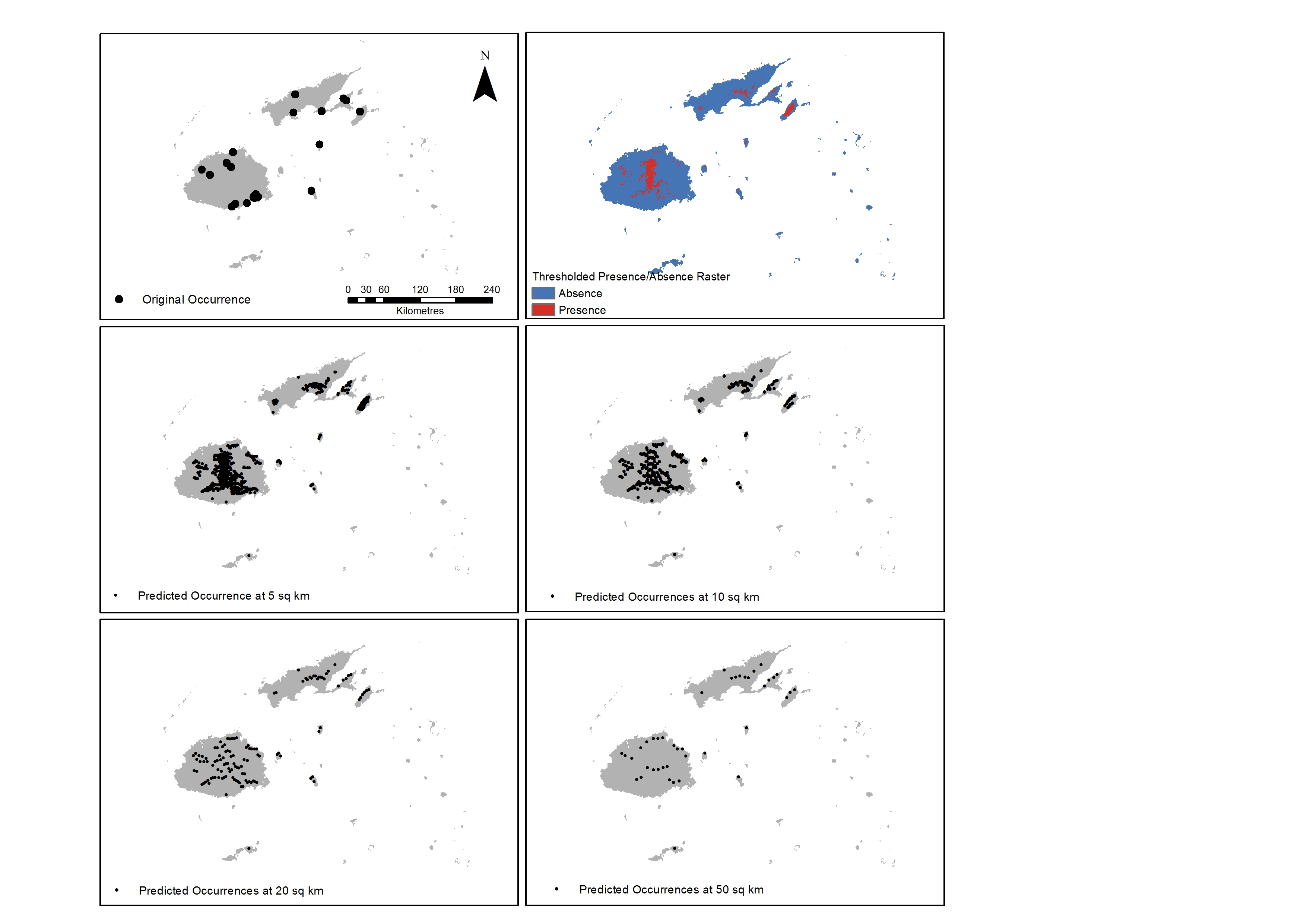
Figure 2. Results of initial run using RF and Mahalanobis with original occurrence points (top left); thresholded rasters (top right) and the resulting spatially rarefied points at a density distribution of 5, 10, 20 and 50 square kilometres (sq km).
When the models were run with increased occurrence numbers, the AUC changed significantly, with all of the models reporting values greater than 0.8. The Kappa values reflected a movement from 0, an indication of better model performance in predicting results as discussed in Allouche et al. (2008). TSS values also improved with sample sizes bigger than the original occurrence set (Tables 2, 3, 4). With the bigger occurrence sizes, RF, MaxEnt and SVM became the best performers, an indication that machine-learning algorithms require bigger sample sizes (Hernandez et al., 2006). Likewise, the ranking of Bioclim and Domain as having the lowest performance and the regression methods GLM and Mahalanobis at intermediate-level performance was confirmed (Wisz et al., 2008; Duan et al., 2014).
| Distance (No of pts) | Bioclim | Domain | Mahalanobis | GLM | SVM | RF | MaxEnt | Average |
| Original (24) | 0.706 | 0.630 | 0.901 | 0.749 | 0.871 | 0.931 | 0.722 | 0.787 |
| 50K (44) | 0.797 | 0.821 | 0.906 | 0.921 | 0.901 | 0.944 | 0.931 | 0.889 |
| 20K (124) | 0.868 | 0.777 | 0.877 | 0.906 | 0.906 | 0.930 | 0.924 | 0.884 |
| 10K (261) | 0.886 | 0.803 | 0.907 | 0.922 | 0.928 | 0.929 | 0.933 | 0.901 |
| 5K (646) | 0.899 | 0.824 | 0.922 | 0.932 | 0.939 | 0.937 | 0.937 | 0.913 |
| Average | 0.831 | 0.771 | 0.903 | 0.886 | 0.909 | 0.934 | 0.889 |
Table 2. AUC for different distances and models.
| Distance (No of pts) | Bioclim | Domain | Mahalanobis | GLM | SVM | RF | MaxEnt | Average |
| Original (24) | 0.140 | 0.040 | 0.173 | 0.079 | 0.138 | 0.240 | 0.068 | 0.125 |
| 50K (44) | 0.052 | 0.037 | 0.176 | 0.078 | 0.135 | 0.241 | 0.068 | 0.112 |
| 20K (124) | 0.099 | 0.185 | 0.211 | 0.211 | 0.124 | 0.241 | 0.338 | 0.201 |
| 10K (261) | 0.361 | 0.221 | 0.306 | 0.316 | 0.928 | 0.929 | 0.933 | 0.571 |
| 5K (646) | 0.402 | 0.306 | 0.417 | 0.414 | 0.421 | 0.461 | 0.406 | 0.404 |
| Average | 0.211 | 0.158 | 0.257 | 0.220 | 0.349 | 0.422 | 0.363 |
Table 3. Kappa averages for each distance and model.
| Distance (No of pts) | Bioclim | Domain | Mahalanobis | GLM | SVM | RF | MaxEnt | Average |
| Original (24) | 0.138 | 0.122 | 0.401 | 0.246 | 0.348 | 0.575 | 0.219 | 0.293 |
| 50K (44) | 0.256 | 0.293 | 0.402 | 0.422 | 0.431 | 0.522 | 0.425 | 0.393 |
| 20K (124) | 0.341 | 0.290 | 0.374 | 0.403 | 0.403 | 0.489 | 0.413 | 0.388 |
| 10K (261) | 0.385 | 0.302 | 0.408 | 0.419 | 0.433 | 0.425 | 0.417 | 0.398 |
| 5K (646) | 0.406 | 0.319 | 0.434 | 0.431 | 0.436 | 0.473 | 0.417 | 0.417 |
| Average | 0.305 | 0.265 | 0.404 | 0.384 | 0.410 | 0.497 | 0.378 |
Table 4. TSS averages for each distance and model.
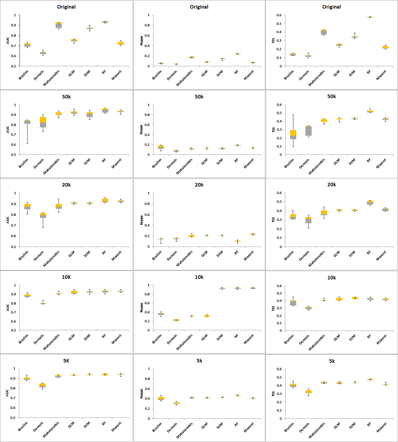
Figure 3. Plots of AUC, Kappa and TSS per distance for all algorithms.
The CV shows that the Domain and Bioclim algorithms were the least consistent across all three performance metrics (AUC, Kappa and TSS). RF showed the greatest consistency when its CV was plotted against AUC while SVM was most consistent when the CV plotted against Kappa and TSS. The machine learning algorithms MaxEnt, SVM and RF had considerably greater consistency compared to the other groups. GLM was also more consistent than the Mahalanobis model. Based on the AUC and Kappa performance of the models at different distances (Figure 3) and the CV (Figure 4), the rarefication distance result at 10 kilometre distance consisting of 261 points was selected because it provided the best performance and consistency (Tables 2-4 and Figure 3). This is consistent with related work that showed better performance at higher sampling points (Bean et al., 2011; Stockwell & Peterson, 2002; Hernandez et al., 2006; Wisz et al., 2008).
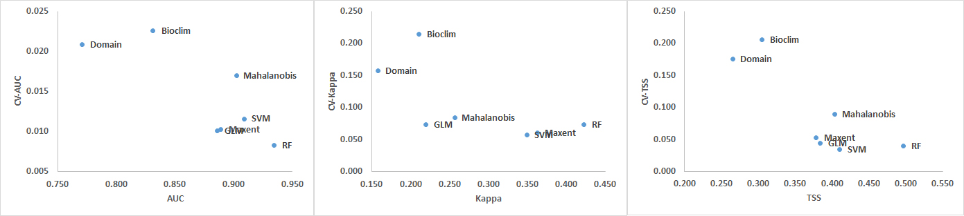
Figure 4. Coefficients of Variation (CV) for AUC, Kappa and TSS averaged over all models (top) and distances (bottom).
Suitability maps for all the algorithms were produced to compare their outputs and, except for the results of Domain, the maps show the central region of Viti Levu and the central ridge of Vanua Levu as the most suitable area for Cerambycidae (Figure 5). The best algorithms for the best-performing distance of 10 kilometres were determined to be the machine-learning methods SVM, randomForest and MaxEnt. This is consistent with the findings reporting better performance of RF, SVM and MaxEnt (Duan et al., 2014; Fukuda et al., 2013). When the weighted ensemble was produced, the areas best suited were on the lower to middle slopes of the central mountains of Viti Levu and the middle slopes of Vanua Levu and Taveuni. These are currently the more heavily forested areas, with higher levels of precipitation compared to the rest of the archipelago.
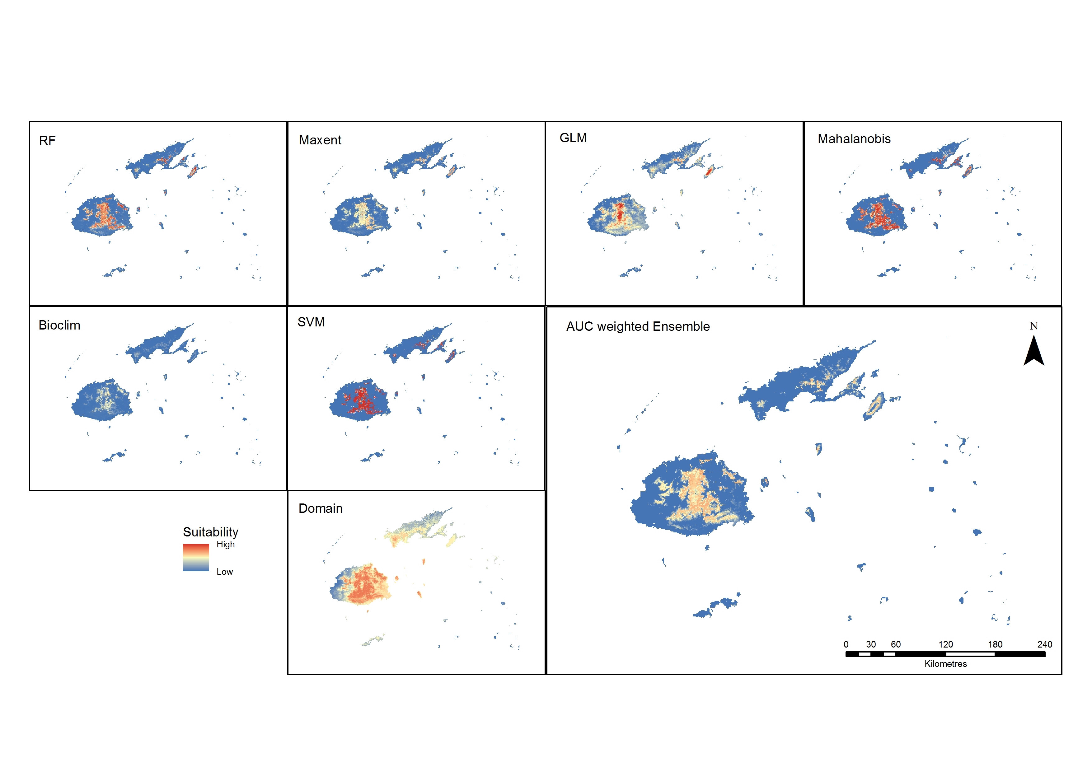
Figure 5. Predicted outputs of all models and the ensemble suitability map from the best performing models (RF, SVM and MaxEnt).
The improvement in model performance resulting from the increase in the number of occurrence points as input to the model is an expected output consistent with previous research efforts (Wisz et al., 2008; MacPherson et al., 2004; Hanberry et al., 2012). Our results confirm the need for adequate occurrence sample sizes based on different modelling approaches; and in cases where additional surveys are difficult or resource-intensive, this offers an alternative method to produce additional, albeit virtual, occurrence points that can make possible the application of a wider range of modelling tools and the improvement of their performance when compared to smaller input occurrences. Using spatial rarefication on larger sample sizes from predicted points is similar to the approach used by Howard et al. (2012) and Kumar, Graham,West, & Evangelista (2014) to eliminate spatial autocorrelation, and provided a more systematic distribution of occurrence points. This approach mitigates data deficiencies associated with lack of resources to conduct further detailed sampling.
The use of the best-performing models, all with AUC greater than 0.9, is an attempt to ensure that the best-performing models produce the best possible sets of data for the next stage. At the selected spatial distance of 10 kilometres (with 261 occurrence points), all the models produced AUC values exceeding 0.7 with Domain as the worst-performing and MaxEnt as the best-performing algorithm. The range of resulting AUCs from 0.823 to 0.937 also showed a narrower range of performance compared to the initial AUC of 0.630 to 0.931. This result also holds true for Kappa and TSS with a slight variation in Kappa where Mahalanobis and GLM are below the values of MaxEnt, RF and SVM. Lower values of the Coefficient of Variation indicated an improvement in performance consistency, justified the increase in sample size and also provided a comparison between algorithms and distribution densities.
Except for Domain results that showed a much wider area of suitability, all the models predicted a similar pattern, with the central area of Viti Levu and the lower half of Vanua Levu as the more favourable sites. These areas are also distinctly vegetated or forested in an area with higher levels of precipitation. The RF and MaxEnt prediction of suitability is similar in coverage, with MaxEnt displaying more uniformity with a lesser range of suitable areas. The GLM output map shows a wider suitability area with a higher range of values in the centre, where the altitude is higher. Mahalanobis and SVM show greater suitability values, while Bioclim shows a low range of suitability.
The ensembled results of the highest-performing models show that the surrounding areas around the higher elevations of the eastern side of Viti Levu have a higher suitability than other areas. Only a small area of Vanua Levu is suitable, which is located in the forested mid-elevation part of the island. The island next to it, Taveuni, shows suitability around the mid-elevation areas. This altitudinal characteristic is consistent with the finding of Waqa-Sakiti and Winder (2012), where elevation was found to have an effect on the spatial distribution of Cerambycidae.
This study provides a method that results in better model performance as reported by standard measurement metrics without employing significant manipulation of options available in each modelling tool (such as regularisation in MaxEnt or the adjustment of the number of background points for all algorithms). Using the predicted presence as input for a second-stage modelling process using multiple high-performing models also opens an opportunity to predict suitability with different conditions, including climate-change-related bioclimatic layers. The availability of future climatic scenarios provides the ability to create models for predicting the suitability of Cerambycidae, and other important organisms, that can provide input to management planning for biodiversity conservation. Overall, this effort provides a basis for further work and in the use of modelling approaches as a complementary tool to much-needed actual field surveys and assessment required for supporting conservation-related efforts and initiatives.
Acknowledgements
Thanks to the Environmental and Animal Sciences Writing Group for providing last-minute assistance, the University of the South Pacific specifically the South Pacific Herbarium for providing access to available data and Unitec e-Press for the support.
References
Aguilar, G.D., Farnworth, M.J., Winder, L. (2015). Mapping the stray domestic cat (Felis catus) population in New Zealand: Species distribution modelling with a climate change scenario and implications for protected areas. Applied Geography 63, pp. 146–154. doi:10.1016/j.apgeog.2015.06.019
Allouche, .O, Tsoar, A., Kadmon, R. (2006). Assessing the accuracy of species distribution models: prevalence, kappa and the true skill statistic (TSS). Journal of Applied Ecology, 43(6), pp. 1223–1232. doi:10.1111/j.1365-2664.2006.01214.x
Araujo, M., New, M. (2007). Ensemble forecasting of species distributions. Trends in Ecology & Evolution 22(1), pp. 42–47. doi:10.1016/j.tree.2006.09.010
Bombi, P., Salvi, D., Vignoli, L., Bologna, M.A. (2009). Modelling Bedriaga’s rock lizard distribution in Sardinia: An ensemble approach. Amphibia-Reptilia, 30(3), pp. 413–424. doi: 10.1163/156853809788795173
Booth, T.H., Nix, H.A., Busby, J.R., Hutchinson, M.F. (2014). BIOCLIM the first species distribution modelling package, its early applications and relevance to most current MaxEnt studies. Diversity and Distributions, 20(1), pp. 1–9. doi:10.1111/ddi.12144
Boria, R.A., Olson, L.E., Goodman, S.M., Anderson, R.A. (2014). Spatial filtering to reduce sampling bias can improve the performance of ecological niche models. Ecological Modeling, 275, pp. 73-77.
Breiman, L. (2001). Random Forests. Machine Learning 45, pp. 5-32.
Brotons, L., Thuiller, W., Araújo, M.B., Hirzel, A.H. (2004). Presence-absence versus presence-only modelling methods for predicting bird habitat suitability. Ecography 27(4), pp. 437–448. doi:10.1111/j.0906-7590.2004.03764.x
Brown, J.L. (2014). SDMtoolbox: a python-based GIS toolkit for landscape genetic, biogeographic and species distribution model analyses. Methods in Ecology and Evolution, 5(7), pp. 694-700. doi:10.1111/2041-210X.12200
Burges, C.J. (1998). A tutorial on support vector machines for pattern recognition. Data mining and Knowledge Discovery, 2(2), pp. 121–167.
Carpenter, G., Gillson, A.N., Winter, J. (1993). DOMAIN: a flexible modeling procedure for mapping potential distributions of plants and animals. Biodiversity and Conservation, 2, pp. 667-680.
Cayuela, L. (2004). Habitat evaluation for the Iberian wolf Canis lupus in Picos de Europa National Park, Spain. Applied Geography, 24(3), pp. 199–215. doi:10.1016/j.apgeog.2004.04.003
Cheaib, A., Badeau, V., Boe, J., Chuine, I., Delire, C., Dufrêne, E., François, C., Gritti, E.S., Legay, M., Pagé, C., Thuiller, W. (2012). Climate change impacts on tree ranges: Model intercomparison facilitates understanding and quantification of uncertainty. Ecology Letters, 15(6), pp. 533-544. doi: 10.1111/j.1461-0248.2012.01764.x
Chefaoui R.M., Hortal J., Lobo J.M. (2005). Potential distribution modelling, niche characterization and conservation status assessment using using GIS tools: A case study of Iberian Copris species. Biological Conservation 122, pp. 327-338.
Domisch, S., Araújo, M.B., Bonada, N., Pauls, S.U., Jähnig, S.C., Haase, P. (2013). Modelling distribution in European stream macroinvertebrates under future climates. Global Change Biology 19(3), pp. 752–762. doi:10.1111/gcb.12107
Dormann, C.F., Elith, J., Bacher, S., Buchmann C., Carl, G., Carre, G., Marquez, J.R.G., Gruber, B., Lafourcade, B., Leitao, P.J., Munkemuller, T., McClean, C., Osborne, P.E., Reineking, B., Schroder, B., Skidmore, A.K., Zurell, D., Lautenbach, S. (2013). Collinearity: a review of methods to deal with it and a simulation study evaluating their performance. Ecography, 36(1), pp. 27–46.
Drake, J.M., Randin, C., Guisan, A. (2006). Modelling ecological niches with support vector machines. Journal of Applied Ecology, 43, pp. 424–432.
Duan, R.Y., Kong, X.Q., Huang, M.Y., Fan, W.Y., Wang, Z.G. (2014). The predictive performance and stability of six species distribution models. PloS One, 9(11), p. e112764. doi:10.1371/journal.pone.0112764
Elith, J., Burgman, M.A., Regan, H.M. (2002). Mapping epistemic uncertainties and vague concepts in predictions of species distribution. Ecological Modelling, 157, pp. 313–329.
Elith, J., Graham, H.C., Anderson, P.R., Dudík, M., Ferrier, S., Guisan, A., Zimmermann, N.E. (2006). Novel methods improve prediction of species’ distributions from occurrence data. Ecography, 29(2), pp. 129–151. http://doi.org/10.1111/j.2006.0906-7590.04596.x
Evangelista, P.H., Norman, J., Berhanu, L., Kumar, S., & Alley, N. (2008). Predicting habitat suitability for the endemic mountain nyala (Tragelaphus buxtoni) in Ethiopia. Wildlife Research, 35(5), pp. 409-416. doi: 10.1071/WR07173
Evans, J.M., Fletcher, R.J., Alavalapati, J. (2010). Using species distribution models to identify suitable areas for biofuel feedstock production. GCB Bioenergy, 2(2), pp. 63–78. doi:10.1111/j.1757-1707.2010.01040.x
Faleiro, F.V., Machado, R.B., Loyola, R.D. (2013). Defining spatial conservation priorities in the face of land-use and climate change. Biological Conservation, 158, pp. 248–257. doi:10.1016/j.biocon.2012.09.020
Feeley, K.J., Hurtado, J., Saatchi, S., Silman, M.R., Clark, D.B. (2013). Compositional shifts in Costa Rican forests due to climate-driven species migrations. Global Change Biology, 19(11), pp. 3472–3480. doi:10.1111/gcb.12300
Ferrier, S., Watson, G. (1997). An evaluation of the effectiveness of environmental surrogates and modelling techniques in predicting the distribution of biological diversity. Environment Australia: Canberra
Fitzpatrick, M.C., Sanders, N.J., Ferrier, S., Longino, J.T., Weiser, M.D., Dunn, R. (2011). Forecasting the future of biodiversity: A test of single- and multi-species models for ants in North America. Ecography, 34(5), pp. 836–847. doi:10.1111/j.1600-0587.2011.06653.x
Foody, G.M., Campbell, N.A., Trodd, N.M., Wood, T.F. (1992). Derivation and applications of probabilistic measures of class membership from the maximum-likelihood classification. Photogrammetric Engineering and Remote Sensing, 58(9), pp. 1335-1341.
Fourcade, Y., Engler, J.O., Rödder, D., Secondi, J. (2014). Mapping species distributions with MAXENT using a geographically biased sample of presence data: a performance assessment of methods for correcting sampling bias. PloS One, 9(5), p. e97122. doi:10.1371/journal.pone.0097122
Fukuda, S., De Baets, B., Waegeman, W., Verwaeren, J., Mouton, A.M. (2013). Habitat prediction and knowledge extraction for spawning European grayling (Thymallus thymallus L.) using a broad range of species distribution models. Environmental Modelling and Software, 47, pp. 1–6. doi:10.1016/j.envsoft.2013.04.005
Guillera-Arroita, G., Lahoz-Monfort, J.J., Elith, J., Gordon, A., Kujala, H., Lentini, P.E., McCarthy, M.A., Tingley, R., Wintle, B.A. (2015). Is my species distribution model fit for purpose? Matching data and models to applications. Global Ecology and Biogeography, 24(3), pp. 276-292.
Guisan, A., Edwards, T.C., Hastie, T. (2002). Generalized linear and generalized additive models in studies of species distributions: setting the scene. Ecological Modelling, 157, pp. 89–100. doi: 10.1016/S0304-3800(02)00204-1
Guisan, A., Tingley, R., Baumgartner, J.B., Naujokaitis-Lewis, I., Sutcliffe, P.R., Tulloch, A.I.T., Regan, T.J., Brotons, L., McDonald-Madden, E., Mantyka-Pringle, C., Martin, T.G. (2013). Predicting species distributions for conservation decisions. Ecology Letters, 16, pp. 1424–1435. doi:10.1111/ele.12189
Guo, Q., Liu, Y. (2010). ModEco: an integrated software package for ecological niche modelling. Ecography, 33(4), pp. 637–642. doi:10.1111/j.1600-0587.2010.06416.x
Guo, Q., Kelly, M., Graham, C. (2005). Support vector machines for predicting distribution of Sudden Oak Death in California. Ecological Modelling, 182, pp. 75-90.
Hanberry, B.B., He, H.S., Dey, D.C. (2012). Sample sizes and model comparison metrics for species distribution models. Ecological Modelling, 227, pp. 29-33.
Hernandez, P.A., Graham, C.H., Master, L.L., Albert, D.L. (2006). The effect of sample size and species characteristics on performance of different species distribution modelling methods. Ecography 29(5), pp. 773–785. doi:10.1111/j.0906-7590.2006.04700.x
Higgins, P.A. (2007). Biodiversity loss under existing land use and climate change: an illustration using northern South America. Global Ecology and Biogeography, 16(2), pp. 197-204.
Hijmans, R.J., Cameron, S.E., Parra, J.L., Jones, P.G., Jarvis, A. (2005). Very high resolution interpolated climate surfaces for global land areas. International Journal of Climatology, 25(15), pp. 1965–1978. doi:10.1002/joc.1276
Hijmans, R.J., Phillips, S., Leathwick, J., Elith., J, (2013). dismo: Species distribution modelling. R package version 0.8-11.
Hijmans, R.J., Elith, J. (2016). Species distribution modelling with R.Hijmans, R.J. (2012). Cross-validation of species distribution models: removing spatial sorting bias and calibration with a null model. Ecology 93, pp. 679–688.
Howard, A.M., Bernardes, S., Nibbelink, N., Biondi, L., Presotto, A., Fragaszy, D.M., Madden, M. (2012). A maximum entropy model of the bearded capuchin monkey habitat incorporating topography and spectral unmixing analysis. In ISPRS Annals of the Photogrammetry, Remote Sensing and Spatial Information Sciences, 2012 XXII ISPRS congress, 25 August-01 September, Melbourne, Australia, (I-2):7-11.
Jarnevich, C.S., Stohlgren, T.J. (2009). Near term climate projections for invasive species distributions. Biological Invasions, 11(6), pp. 1373–1379. doi:10.1007/s10530-008-9345-8
Jarnevich, C.S., Stohlgren, T.J., Kumar, S., Morisette, J.T., Holcombe, T.R. (2015). Caveats for correlative species distribution modelling. Ecological Informatics, 29, pp. 6–15. doi:10.1016/j.ecoinf.2015.06.007
Lambin, E.F., Meyfroidt, P. (2011). Global land use change, economic globalization, and the looming land scarcity. Proceedings of the National Academy of Sciences, 108(9), pp. 3465-3472.
Liang, L., Clark, J.T., Kong, N., Rieske, L.K., Fei, S. (2014). Spatial analysis facilitates invasive species risk assessment. Forest Ecology and Management, 315, pp. 22–29. doi:10.1016/j.foreco.2013.12.019
Lobo, J.M., Jimenez-Valverde, A., Real, R. (2008). AUC: a misleading measure of the performance of predictive distribution models. Global Ecology and Biogeography, 17, pp. 145–151.
Kramer-Schadt, S., Niedballa, J., Pilgrim, J.D., Schröder, B., Lindenborn, J., Reinfelder, V., Stillfried, M., Heckmann, I., Scharf, A.K., Augeri, D.M., Cheyne, S.M. (2013). The importance of correcting for sampling bias in MaxEnt species distribution models. Diversity and Distributions, 19(11), pp. 1366-1379. doi:10.1111/ddi.12096
Kumar, S., Graham, J., West, A. M., & Evangelista, P. H. (2014). Using district-level occurrences in MaxEnt for predicting the invasion potential of an exotic insect pest in India. Computers and Electronics in Agriculture 103, pp. 55-62. http:// dx.doi.org/10.1016/j.compag.2014.02.007.
Liu, C., White, M., Newell, G. (2013). Selecting thresholds for the prediction of species occurrence with presence-only data. Journal of Biogeography, 40(4), pp. 778–789. doi:10.1111/jbi.12058
Mahalanobis, P.C. (1936). On the generalised distance in statistics. Proceedings of the National Institute of Sciences of India, 2(1), pp. 49–55.
Marmion, M., Parviainen, M., Luoto, M., Heikkinen, R.K., Thuiller, W. (2009). Evaluation of consensus methods in predictive species distribution modelling. Diversity and Distributions, 5, pp. 59–69.
McPherson, J.M., Jetz, W., Rogers, D.J. (2004). The effects of species’ range sizes on the accuracy of distribution models: ecological phenomena or statistical artefact? Journal of Applied Ecology, 41, pp. 811–823.
Meggs, J.M., Munks, S.A., Corkrey, R., Richards, K. (2004). Development and evaluation of predictive habitat models to assist the conservation planning of a threatened lucanid beetle, Hoplogonus simsoni, in north-east Tasmania. Biological Conservation, 118, pp. 501-511.
Naimi, B., Araújo, M.B. (2016). sdm: a reproducible and extensible R platform for species distribution modelling. Ecography, 39, pp. 368–375.
Nabout, J.C., Soares, T.N., Diniz-Filho, J.A.F., De Marco Júnior, P., Telles, M.P.C., Naves, R.V., Chaves, L.J. (2010). Combining multiple models to predict the geographical distribution of the Baru tree (Dipteryx alata Vogel) in the Brazilian Cerrado. Brazilian Journal of Biology, 70(4), pp. 911–919. http://www.ncbi.nlm.nih.gov/pubmed/21180894 (In Portuguese)
Oleas, N.H., Meerow, A.W., Feeley, K.J., Gebelein, J., Francisco-Ortega, J. (2014). Using species distribution models as a tool to discover new populations of Phaedranassa brevifolia Meerow, 1987 (Liliopsida: Amaryllidaceae) in Northern Ecuador. Check List, 10(3), pp. 689–691. doi:10.15560/10.3.689
Pearson, R.G., Dawson, T.P., Liu, C. (2004). Modelling species distributions in Britain: a hierarchical integration of climate and land-cover data. Ecography, 27, pp. 285–298.
Peterson, A.T., Martínez-Campos, C., Nakazawa, Y., Martínez-Meyer, E. (2005). Time-specific ecological niche modelling predicts spatial dynamics of vector insects and human dengue cases. Transactions of the Royal Society of Tropical Medicine and Hygiene, 99, pp. 647-655.
Phillips, S.J., Anderson, R.P., Schapire, R.E. (2006). Maximum entropy modelling of species geographic distributions. Ecological Modelling, 190(3-4), pp. 231–259. doi:10.1016/j.ecolmodel.2005.03.026
Poulos, H., Chernoff, B., Fuller, P., Butman, D. (2012). Ensemble forecasting of potential habitat for three invasive fishes. Aquatic Invasions, 7(1), pp. 59–72. doi:10.3391/ai.2012.7.1.007
Puschendorf, R., Carnaval, A.C., VanDerWal, J., Zumbado-Ulate, H., Chaves, G., Bolaños, F., Alford, R.A. (2009). Distribution models for the amphibian chytrid Batrachochytrium dendrobatidis in Costa Rica: proposing climatic refuges as a conservation tool. Diversity and Distributions, 15(3), pp. 401–408. doi:10.1111/j.1472-4642.2008.00548.x
Raxworthy, C.J., Martınez-Meyer, E., Horning, N., Nussbaum, R.A., Schneider, G.E., Ortega-Huerta, M.A., Peterson, A.T. (2003). Predicting distributions of known and unknown reptile species in Madagascar. Nature, 426, pp. 837–841.
Raybaud, V., Beaugrand, G., Dewarumez, J.M., Luczak, C. (2015). Climate-induced range shifts of the American jackknife clam Ensis directus in Europe. Biological Invasions, 17(2), pp. 725-741.
Roura-Pascual, N., Brotons, L., Peterson, A.T., Thuiller, W. (2008). Consensual predictions of potential distributional areas for invasive species: a case study of Argentine ants in the Iberian Peninsula. Biological Invasions, 11(4), pp. 1017–1031. doi:10.1007/s10530-008-9313-3
Rodriguez, J.P., Brotons, L., Bustamante, J., Seoane, J. (2007). The application of predictive modelling of species distribution to biodiversity conservation. Diversity & Distributions, 13(3), pp. 243-251. doi:10.1111/j.1472-4642.2007.00356.x
Rushton, S.P., Ormerod, S.J., Kerby, G. (2004). New paradigms for modelling species distributions? Journal of Applied Ecology, 41, pp. 193–200. doi:10.1111/j.0021-8901.2004.00903.x
Sauer, J., Domisch, S., Nowak, C., Haase, P. (2011) . Low mountain ranges: summit traps for montane freshwater species under climate change. Biodiversity and Conservation, 20(13), pp. 3133–3146. doi:10.1007/s10531-011-0140-y
Segurado, P., Araujo, M.B. (2004). An evaluation of methods for modelling species’ distributions. Journal of Biogeography, 31, pp. 1555–1568.
de Souza Muñoz, M.E., De Giovanni, R., de Siqueira, M.F., Sutton, T., Brewer, P., Pereira, R.S., Canhos, D.A.L., Canhos, V.P. (2011). openModeller: a generic approach to species’ potential distribution modelling. GeoInformatica, 15(1), pp. 111-135.
Stockwell, D.R., Peterson, A.T. (2002). Effects of sample size on accuracy of species distribution models. Ecological Modelling, 148(1), pp. 1–13. doi:10.1016/S0304-3800(01)00388-X
Stohlgren, T.J., Ma, P., Kumar, S., Rocca, M., Morisette, J.T., Jarnevich, C.S., Benson, N. (2010). Ensemble habitat mapping of invasive plant species. Risk Analysis: An Official Publication of the Society for Risk Analysis, 30(2), pp. 224–35. doi:10.1111/j.1539-6924.2009.01343.x
Thuiller, W., Richardson, D. (2005). Niche-based modelling as a tool for predicting the risk of alien plant invasions at a global scale. Global Change Biology, 11, pp. 2234–2250. doi:10.1111/j.1365-2486.2005.01018.x
Thuiller, W., Lafourcade, B., Engler, R., Araújo, M.B. (2009). BIOMOD – a platform for ensemble forecasting of species distributions. Ecography, 32(3), pp. 369–373. doi:10.1111/j.1600-0587.2008.05742.x
Tognelli, M.F., Roig-Juñent, S.A., Marvaldi, A.E., Flores, G.E., Lobo, J.M. (2009). An evaluation of methods for modelling distribution of Patagonian insects. Revista Chilena de Historia Natural, 82(3): 347–360. doi:10.4067/S0716-078X2009000300003
Veloz, S.D. (2009). Spatially autocorrelated sampling falsely inflates measures of accuracy for presence- only niche models. Journal of Biogeography, 36, pp. 2290–2299.
Warner, M. (2000). Conflict management in community-based natural resource projects: experiences from Fiji and Papua New Guinea. London, UK: Overseas Development Institute. Retrieved from: http://citeseerx.ist.psu.edu/viewdoc/download?doi=10.1.1.168.4002&rep=rep1&type=pdf
Waqa-Sakiti, H., Winder, L. (2012). Diversity and distribution of forest canopy Coleoptera on eastern Viti Levu, Fiji Islands. Pacific Conservation Biology, 18(3), pp. 177-185.
Wilson, J.R.U., Richardson, D.M., Rouget, M., Proches, S., Amis, M.A., Henderson, L., Thuiller, W. (2007). Residence time and potential range: crucial considerations in modelling plant invasions. Diversity and Distributions, 13, pp. 11–22.
Wisz, M.S., Hijmans, R.J., Li, J., Peterson, A.T., Graham, C.H., Guisan, A. (2008 ). Effects of sample size on the performance of species distribution models. Diversity and Distributions, 14(5), pp. 763–773. doi:10.1111/j.1472-4642.2008.00482.x
Yates, C.J., Elith, J., Latimer, A.M., Le Maitre, D., Midgley, G.F., Schurr, F.M., West, A.G. (2009). Projecting climate change impacts on species distributions in megadiverse South African Cape and Southwest Australian Floristic Regions: Opportunities and challenges. Austral Ecology, 35(4), pp. 374–391. doi:10.1111/j.1442-9993.2009.02044.x
Zhang, L., Liu, S., Sun, P., Wang, T., Wang, G., Zhang, X., Wang, L. (2015). Consensus forecasting of species distributions: The effects of niche model performance and niche properties. PLoS ONE, 10(3), pp. 1–18. doi:10.1371/journal.pone.0120056
Author’s Bios
Glenn Aguilar is a Senior Lecturer in Environmental and Animal Sciences of the Unitec Institute of Technology. His research and teaching interests include Geographic Information Systems and its applications in biodiversity conservation and animal management, climate change modelling, species distribution modelling, risk assessment, citizen science and agent based design and modelling.
Contact gaguilar@unitec.ac.nz
Hilda Waqa-Sakiti is a Research Fellow at the South Pacific Herbarium of the Institute of Applied Science of the University of the South Pacific. She worked on the taxonomy, phylogenetics and biogeography of the Fijian long-horned beetle for her PhD thesis at the University of the South Pacific.
Contact hilda.waqa@gmail.com
Linton Winder is Head of Forestry and Resource Management at Toi Ohomai Institute of Technology in Rotorua. He is an entomologist with a background in agricultural and forest ecology. He has worked around the world – in the UK, Fiji, New Zealand and briefly Mauritius. Current projects include a partnership with the Biological Husbandry Unit and Lincoln University focussing on the tomato potato psyllid, and working with colleagues in Fiji at the University of the South Pacific on a number of forest conservation projects.
Contact linton.winder@toiohomai.ac.nz
Using Predicted Locations and an Ensemble Approach to Address Sparse Data Sets for Species Distribution Modelling: Long-horned Beetles (Cerambycidae) of the Fiji Islands, by Glenn D. Aguilar, Hilda Waqa-Sakiti and Linton Winder, is licensed under a Creative Commons Attribution-NonCommercial 4.0 International License.
To cite this report correctly, please refer to imprint page information on the the pdf version.